
![Coursera: Neural Networks and Deep Learning (Week 4.1) [Assignment Solution] - deeplearning.ai | APDaga | DumpBox](https://blogger.googleusercontent.com/img/b/R29vZ2xl/AVvXsEgs2yfKQRp8W1_VLlONcTzij2YNs9wEWybleC7E5sqzpD3lvrS6-7KGdtIIoQfduIuOGmDMZ8bD9T3leNe0-kaeINzELlgODdFnzDjKwaQrtFZXVlH_0gXsVCTWY-HeYvrCiIa5HXD65TU/s320/NN+week4.1+thumbnail-min.jpg "Coursera: Neural Networks and Deep Learning (Week 4.1) [Assignment Solution] - deeplearning.ai | APDaga | DumpBox")
▸ Building your Deep Neural Network: Step by Step.
I have recently completed the Neural Networks and Deep Learning course from Coursera by deeplearning.ai
While doing the course we have to go through various quiz and assignments in Python.
Here, I am sharing my solutions for the weekly assignments throughout the course.
> It is recommended that you should solve the assignments by yourself honestly then only it makes sense to complete the course.
> But, In case you stuck in between, feel free to refer to the solutions provided by me.
![Coursera: Neural Networks and Deep Learning (Week 4.1) [Assignment Solution] - deeplearning.ai | APDaga | DumpBox](https://blogger.googleusercontent.com/img/b/R29vZ2xl/AVvXsEgs2yfKQRp8W1_VLlONcTzij2YNs9wEWybleC7E5sqzpD3lvrS6-7KGdtIIoQfduIuOGmDMZ8bD9T3leNe0-kaeINzELlgODdFnzDjKwaQrtFZXVlH_0gXsVCTWY-HeYvrCiIa5HXD65TU/s1600/NN+week4.1+thumbnail-min.jpg "Coursera: Neural Networks and Deep Learning (Week 4.1) [Assignment Solution] - deeplearning.ai | APDaga | DumpBox") |
I have recently completed the Neural Networks and Deep Learning course from Coursera by deeplearning.ai
NOTE:
Don't just copy paste the code for the sake of completion. Even if you copy the code, make sure you understand the code first.
Click here: Coursera: Neural Networks & Deep Learning (Week 3)
Click Here: Coursera: Neural Networks & Deep Learning (Week 4B)
Scroll down for Coursera: Neural Networks & Deep Learning (Week 4A) Assignments.
Recommended Machine Learning Courses:- Coursera: Machine Learning
- Coursera: Deep Learning Specialization
- Coursera: Machine Learning with Python
- Coursera: Advanced Machine Learning Specialization
- Udemy: Machine Learning
- LinkedIn: Machine Learning
- Eduonix: Machine Learning
- edX: Machine Learning
- Fast.ai: Introduction to Machine Learning for Coders
Even if you copy the code, make sure you understand the code first.
Click Here: Coursera: Neural Networks & Deep Learning (Week 4B)
Scroll down for Coursera: Neural Networks & Deep Learning (Week 4A) Assignments.
- Coursera: Machine Learning
- Coursera: Deep Learning Specialization
- Coursera: Machine Learning with Python
- Coursera: Advanced Machine Learning Specialization
- Udemy: Machine Learning
- LinkedIn: Machine Learning
- Eduonix: Machine Learning
- edX: Machine Learning
- Fast.ai: Introduction to Machine Learning for Coders
Building your Deep Neural Network: Step by Step
- In this notebook, you will implement all the functions required to build a deep neural network.
- In the next assignment, you will use these functions to build a deep neural network for image classification.
After this assignment you will be able to:- Use non-linear units like ReLU to improve your model
- Build a deeper neural network (with more than 1 hidden layer)
- Implement an easy-to-use neural network class
Notation:- Superscript denotes a quantity associated with the layer.
- Example: is the layer activation. and are the layer parameters.
- Superscript denotes a quantity associated with the example.
- Example: is the training example.
- Lowerscript denotes the entry of a vector.
- Example: denotes the entry of the layer's activations).
Let's get started!
- Example: is the layer activation. and are the layer parameters.
- Example: is the training example.
- Example: denotes the entry of the layer's activations).
1 - Packages
Let's first import all the packages that you will need during this assignment.- numpy is the main package for scientific computing with Python.
- matplotlib is a library to plot graphs in Python.
- dnn_utils provides some necessary functions for this notebook.
- testCases provides some test cases to assess the correctness of your functions
- np.random.seed(1) is used to keep all the random function calls consistent. It will help us grade your work. Please don't change the seed.
In [1]:

Figure 1
In [2]:
In [3]:
2 - Outline of the Assignment
To build your neural network, you will be implementing several "helper functions". These helper functions will be used in the next assignment to build a two-layer neural network and an L-layer neural network. Each small helper function you will implement will have detailed instructions that will walk you through the necessary steps. Here is an outline of this assignment, you will:
- Initialize the parameters for a two-layer network and for an -layer neural network.
- Implement the forward propagation module (shown in purple in the figure below).
- Complete the LINEAR part of a layer's forward propagation step (resulting in ).
- We give you the ACTIVATION function (relu/sigmoid).
- Combine the previous two steps into a new [LINEAR->ACTIVATION] forward function.
- Stack the [LINEAR->RELU] forward function L-1 time (for layers 1 through L-1) and add a [LINEAR->SIGMOID] at the end (for the final layer ). This gives you a new L_model_forward function.
- Compute the loss.
- Implement the backward propagation module (denoted in red in the figure below).
- Complete the LINEAR part of a layer's backward propagation step.
- We give you the gradient of the ACTIVATE function (relu_backward/sigmoid_backward)
- Combine the previous two steps into a new [LINEAR->ACTIVATION] backward function.
- Stack [LINEAR->RELU] backward L-1 times and add [LINEAR->SIGMOID] backward in a new L_model_backward function
- Finally update the parameters.
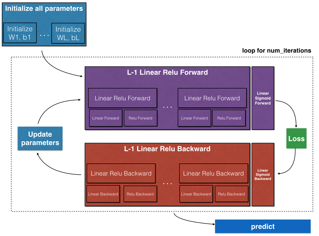
Note that for every forward function, there is a corresponding backward function. That is why at every step of your forward module you will be storing some values in a cache. The cached values are useful for computing gradients. In the backpropagation module you will then use the cache to calculate the gradients. This assignment will show you exactly how to carry out each of these steps.
Check-out our free tutorials on IOT (Internet of Things):
3 - Initialization
You will write two helper functions that will initialize the parameters for your model. The first function will be used to initialize parameters for a two layer model. The second one will generalize this initialization process to layers.
3.1 - 2-layer Neural Network
Exercise: Create and initialize the parameters of the 2-layer neural network.
Instructions:
- The model's structure is: LINEAR -> RELU -> LINEAR -> SIGMOID.
- Use random initialization for the weight matrices. Use
np.random.randn(shape)*0.01with the correct shape. - Use zero initialization for the biases. Use
np.zeros(shape).
In [2]:
# GRADED FUNCTION: initialize_parameters

def initialize_parameters(n_x, n_h, n_y):
    """
    Argument:
    n_x -- size of the input layer
    n_h -- size of the hidden layer
    n_y -- size of the output layer

    Returns:
    parameters -- python dictionary containing your parameters:
                    W1 -- weight matrix of shape (n_h, n_x)
                    b1 -- bias vector of shape (n_h, 1)
                    W2 -- weight matrix of shape (n_y, n_h)
                    b2 -- bias vector of shape (n_y, 1)
    """

    np.random.seed(1)

    ### START CODE HERE ### (≈ 4 lines of code)
    W1 = np.random.randn(n_h,n_x)*0.01
    b1 = np.zeros((n_h,1))
    W2 = np.random.randn(n_y,n_h)*0.01
    b2 = np.zeros((n_y,1))
    ### END CODE HERE ###

    assert(W1.shape == (n_h, n_x))
    assert(b1.shape == (n_h, 1))
    assert(W2.shape == (n_y, n_h))
    assert(b2.shape == (n_y, 1))

    parameters = {"W1": W1,
                  "b1": b1,
                  "W2": W2,
                  "b2": b2}

    return parameters
In [3]:
Out [3]:
Expected output:
W1 | [[ 0.01624345 -0.00611756 -0.00528172] [-0.01072969 0.00865408 -0.02301539]] |
b1 | [[ 0.] [ 0.]] |
W2 | [[ 0.01744812 -0.00761207]] |
b2 | [[ 0.]] |
3.2 - L-layer Neural Network
The initialization for a deeper L-layer neural network is more complicated because there are many more weight matrices and bias vectors. When completing the
initialize_parameters_deep, you should make sure that your dimensions match between each layer. Recall that is the number of units in layer . Thus for example if the size of our input is (with examples) then:
Exercise: Implement initialization for an L-layer Neural Network.
Instructions:
- The model's structure is [LINEAR -> RELU] (L-1) -> LINEAR -> SIGMOID. I.e., it has layers using a ReLU activation function followed by an output layer with a sigmoid activation function.
- Use random initialization for the weight matrices. Use
np.random.randn(shape) * 0.01. - Use zeros initialization for the biases. Use
np.zeros(shape). - We will store , the number of units in different layers, in a variable
layer_dims. For example, thelayer_dimsfor the "Planar Data classification model" from last week would have been [2,4,1]: There were two inputs, one hidden layer with 4 hidden units, and an output layer with 1 output unit. Thus meansW1's shape was (4,2),b1was (4,1),W2was (1,4) andb2was (1,1). Now you will generalize this to layers! - Here is the implementation for (one layer neural network). It should inspire you to implement the general case (L-layer neural network).
In [4]:
In [5]:
Out [5]:
Expected output:
W1 | [[ 0.01788628 0.0043651 0.00096497 -0.01863493 -0.00277388] [-0.00354759 -0.00082741 -0.00627001 -0.00043818 -0.00477218] [-0.01313865 0.00884622 0.00881318 0.01709573 0.00050034] [-0.00404677 -0.0054536 -0.01546477 0.00982367 -0.01101068]] |
b1 | [[ 0.] [ 0.] [ 0.] [ 0.]] |
W2 | [[-0.01185047 -0.0020565 0.01486148 0.00236716] [-0.01023785 -0.00712993 0.00625245 -0.00160513] [-0.00768836 -0.00230031 0.00745056 0.01976111]] |
b2 | [[ 0.] [ 0.] [ 0.]] |
4 - Forward propagation module
4.1 - Linear Forward
Now that you have initialized your parameters, you will do the forward propagation module. You will start by implementing some basic functions that you will use later when implementing the model. You will complete three functions in this order:
- LINEAR
- LINEAR -> ACTIVATION where ACTIVATION will be either ReLU or Sigmoid.
- [LINEAR -> RELU] (L-1) -> LINEAR -> SIGMOID (whole model)
The linear forward module (vectorized over all the examples) computes the following equations:
Z[l]=W[l]A[l−1]+b[l] (4)
where .Exercise: Build the linear part of forward propagation.
Reminder: The mathematical representation of this unit is . You may also find
np.dot() useful. If your dimensions don't match, printing W.shape may help.In [7]:
Out [7]:
Expected output:
| Z | [[ 3.26295337 -1.23429987]] |
4.2 - Linear-Activation Forward
In this notebook, you will use two activation functions:
- Sigmoid: . We have provided you with the
sigmoidfunction. This function returns two items: the activation value "a" and a "cache" that contains "Z" (it's what we will feed in to the corresponding backward function). To use it you could just call:A, activation_cache = sigmoid(Z) - ReLU: The mathematical formula for ReLu is . We have provided you with the
relufunction. This function returns twoitems: the activation value "A" and a "cache" that contains "Z" (it's what we will feed in to the corresponding backward function). To use it you could just call:A, activation_cache = relu(Z)
For more convenience, you are going to group two functions (Linear and Activation) into one function (LINEAR->ACTIVATION). Hence, you will implement a function that does the LINEAR forward step followed by an ACTIVATION forward step.
Exercise: Implement the forward propagation of the LINEAR->ACTIVATION layer. Mathematical relation is: where the activation "g" can be sigmoid() or relu(). Use linear_forward() and the correct activation function.
# GRADED FUNCTION: linear_activation_forward

def linear_activation_forward(A_prev, W, b, activation):
    """
    Implement the forward propagation for the LINEAR->ACTIVATION layer

    Arguments:
    A_prev -- activations from previous layer (or input data): (size of previous layer, number of examples)
    W -- weights matrix: numpy array of shape (size of current layer, size of previous layer)
    b -- bias vector, numpy array of shape (size of the current layer, 1)
    activation -- the activation to be used in this layer, stored as a text string: "sigmoid" or "relu"

    Returns:
    A -- the output of the activation function, also called the post-activation value
    cache -- a python dictionary containing "linear_cache" and "activation_cache";
             stored for computing the backward pass efficiently
    """

    if activation == "sigmoid":
        # Inputs: "A_prev, W, b". Outputs: "A, activation_cache".
        ### START CODE HERE ### (≈ 2 lines of code)
        Z, linear_cache = linear_forward(A_prev, W, b)
        A, activation_cache = sigmoid(Z)
        ### END CODE HERE ###

    elif activation == "relu":
        # Inputs: "A_prev, W, b". Outputs: "A, activation_cache".
        ### START CODE HERE ### (≈ 2 lines of code)
        Z, linear_cache = linear_forward(A_prev, W, b)
        A, activation_cache = relu(Z)
        ### END CODE HERE ###

    assert (A.shape == (W.shape[0], A_prev.shape[1]))
    cache = (linear_cache, activation_cache)
    # linear_cache = (A, W, b)
    # activation_cache = (Z)
    # cache = ((A, W, b), (Z))

    #print("linear_cache = "+ str(linear_cache))
    #print("activation_cache = "+ str(activation_cache))
    #print("cache = "+ str(cache))

    return A, cache
In [9]:
Out [9]:
Expected output:
| With sigmoid: A | [[ 0.96890023 0.11013289]] |
| With ReLU: A | [[ 3.43896131 0. ]] |
Note: In deep learning, the "[LINEAR->ACTIVATION]" computation is counted as a single layer in the neural network, not two layers.
d) L-Layer Model
For even more convenience when implementing the -layer Neural Net, you will need a function that replicates the previous one (
linear_activation_forward with RELU) times, then follows that with one linear_activation_forward with SIGMOID.
Exercise: Implement the forward propagation of the above model.
Instruction: In the code below, the variable
AL will denote . (This is sometimes also called Yhat, i.e., this is .)Tips:
- Use the functions you had previously written
- Use a for loop to replicate [LINEAR->RELU] (L-1) times
- Don't forget to keep track of the caches in the "caches" list. To add a new value
cto alist, you can uselist.append(c).
In [10]:
# GRADED FUNCTION: L_model_forward

def L_model_forward(X, parameters):
    """
    Implement forward propagation for the [LINEAR->RELU]*(L-1)->LINEAR->SIGMOID computation

    Arguments:
    X -- data, numpy array of shape (input size, number of examples)
    parameters -- output of initialize_parameters_deep()

    Returns:
    AL -- last post-activation value
    caches -- list of caches containing:
                every cache of linear_activation_forward() (there are L-1 of them, indexed from 0 to L-1)
    """

    caches = []
    A = X
    L = len(parameters) // 2                  # number of layers in the neural network

    # Implement [LINEAR -> RELU]*(L-1). Add "cache" to the "caches" list.
    for l in range(1, L):
        A_prev = A
        #print("l = "+str(l))
        ### START CODE HERE ### (≈ 2 lines of code)
        W = parameters['W' + str(l)]
        b = parameters['b' + str(l)]
        A, cache = linear_activation_forward(A_prev, W, b, activation = "relu")
        caches.append(cache)
        ### END CODE HERE ###

    # Implement LINEAR -> SIGMOID. Add "cache" to the "caches" list.
    ### START CODE HERE ### (≈ 2 lines of code)
    #print("L = "+str(L))
    W = parameters['W' + str(L)]
    b = parameters['b' + str(L)]
    AL, cache = linear_activation_forward(A, W, b, activation = "sigmoid")
    caches.append(cache)
    ### END CODE HERE ###

    #print("AL_shape = "+str(AL.shape))
    #print("X_shape[1] = "+str(X.shape[1]))

    assert(AL.shape == (1,X.shape[1]))

    return AL, caches
In [11]:
Out [11]:
| AL | [[ 0.03921668 0.70498921 0.19734387 0.04728177]] |
| Length of caches list | 3 |
Great! Now you have a full forward propagation that takes the input X and outputs a row vector containing your predictions. It also records all intermediate values in "caches". Using , you can compute the cost of your predictions.
5 - Cost function
Now you will implement forward and backward propagation. You need to compute the cost, because you want to check if your model is actually learning.
Exercise: Compute the cross-entropy cost , using the following formula:
−1m∑i=1m(y(i)log(a[L](i))+(1−y(i))log(1−a[L](i))) (7)
In [13]:
Out [13]:
Expected Output:
| cost | 0.41493159961539694 |
6 - Backward propagation module
Just like with forward propagation, you will implement helper functions for backpropagation. Remember that back propagation is used to calculate the gradient of the loss function with respect to the parameters.
Reminder:

The purple blocks represent the forward propagation, and the red blocks represent the backward propagation.
Now, similar to forward propagation, you are going to build the backward propagation in three steps:
- LINEAR backward
- LINEAR -> ACTIVATION backward where ACTIVATION computes the derivative of either the ReLU or sigmoid activation
- [LINEAR -> RELU] (L-1) -> LINEAR -> SIGMOID backward (whole model)
6.1 - Linear backward
For layer , the linear part is: (followed by an activation).
Suppose you have already calculated the derivative . You want to get

Exercise: Use the 3 formulas above to implement linear_backward().
In [14]:
In [15]:
Out [15]:
Expected Output:
In [16]:
In [17]:
Out [17]:
Expected output with sigmoid:
Expected output with relu:

Figure 5 : Backward pass
In [19]:
Out [19]:
Expected Output
In [20]:
In [21]:
Out [21]:
In [15]:
Out [15]:
Expected Output:
dA_prev | [[ 0.51822968 -0.19517421] [-0.40506361 0.15255393] [ 2.37496825 -0.89445391]] |
dW | [[-0.10076895 1.40685096 1.64992505]] |
db | [[ 0.50629448]] |
6.2 - Linear-Activation backward
Next, you will create a function that merges the two helper functions:
linear_backward and the backward step for the activation linear_activation_backward.To help you implement
linear_activation_backward, we provided two backward functions:sigmoid_backward: Implements the backward propagation for SIGMOID unit. You can call it as follows:
dZ = sigmoid_backward(dA, activation_cache)
relu_backward: Implements the backward propagation for RELU unit. You can call it as follows:
dZ = relu_backward(dA, activation_cache)
If is the activation function,
sigmoid_backward and relu_backward computedZ[l]=dA[l]∗g′(Z[l]) (11)
Exercise: Implement the backpropagation for the LINEAR->ACTIVATION layer.
In [17]:
Out [17]:
Expected output with sigmoid:
dA_prev | [[ 0.11017994 0.01105339] [ 0.09466817 0.00949723] [-0.05743092 -0.00576154]] |
dW | [[ 0.10266786 0.09778551 -0.01968084]] |
db | [[-0.05729622]] |
Expected output with relu:
dA_prev | [[ 0.44090989 0. ] [ 0.37883606 0. ] [-0.2298228 0. ]] |
dW | [[ 0.44513824 0.37371418 -0.10478989]] |
db | [[-0.20837892]] |
6.3 - L-Model Backward
Now you will implement the backward function for the whole network. Recall that when you implemented the
L_model_forward function, at each iteration, you stored a cache which contains (X,W,b, and z). In the back propagation module, you will use those variables to compute the gradients. Therefore, in the L_model_backward function, you will iterate through all the hidden layers backward, starting from layer . On each step, you will use the cached values for layer to backpropagate through layer . Figure 5 below shows the backward pass.Initializing backpropagation: To backpropagate through this network, we know that the output is, . Your code thus needs to compute
dAL . To do so, use this formula (derived using calculus which you don't need in-depth knowledge of):You can then use this post-activation gradient
dAL to keep going backward. As seen in Figure 5, you can now feed in dAL into the LINEAR->SIGMOID backward function you implemented (which will use the cached values stored by the L_model_forward function). After that, you will have to use a for loop to iterate through all the other layers using the LINEAR->RELU backward function. You should store each dA, dW, and db in the grads dictionary. To do so, use this formula :grads["dW"+str(l)]=dW[l] (15)
For example, for this would store in
grads["dW3"].Exercise: Implement backpropagation for the [LINEAR->RELU] (L-1) -> LINEAR -> SIGMOID model.
In [18]:
# GRADED FUNCTION: L_model_backward

def L_model_backward(AL, Y, caches):
    """
    Implement the backward propagation for the [LINEAR->RELU] * (L-1) -> LINEAR -> SIGMOID group

    Arguments:
    AL -- probability vector, output of the forward propagation (L_model_forward())
    Y -- true "label" vector (containing 0 if non-cat, 1 if cat)
    caches -- list of caches containing:
                every cache of linear_activation_forward() with "relu" (it's caches[l], for l in range(L-1) i.e l = 0...L-2)
                the cache of linear_activation_forward() with "sigmoid" (it's caches[L-1])

    Returns:
    grads -- A dictionary with the gradients
             grads["dA" + str(l)] = ...
             grads["dW" + str(l)] = ...
             grads["db" + str(l)] = ...
    """
    grads = {}
    L = len(caches) # the number of layers
    m = AL.shape[1]
    Y = Y.reshape(AL.shape) # after this line, Y is the same shape as AL

    # Initializing the backpropagation
    ### START CODE HERE ### (1 line of code)
    print("L = "+str(L))
    dAL = - (np.divide(Y, AL) - np.divide(1 - Y, 1 - AL))
    #print("dAL = "+str(dAL))
    #print("#########################")
    ### END CODE HERE ###

    # Lth layer (SIGMOID -> LINEAR) gradients. Inputs: "dAL, current_cache". Outputs: "grads["dAL-1"], grads["dWL"], grads["dbL"]
    ### START CODE HERE ### (approx. 2 lines)
    current_cache = caches[L-1]
    grads["dA" + str(L-1)], grads["dW" + str(L)], grads["db" + str(L)] = linear_activation_backward(dAL, current_cache, activation = "sigmoid")
    print("dA"+ str(L-1)+" = "+str(grads["dA" + str(L-1)]))
    print("dW"+ str(L)+" = "+str(grads["dW" + str(L)]))
    print("db"+ str(L)+" = "+str(grads["db" + str(L)]))
    ### END CODE HERE ###

    # Loop from l=L-2 to l=0
    for l in reversed(range(L-1)):
        # lth layer: (RELU -> LINEAR) gradients.
        # Inputs: "grads["dA" + str(l + 1)], current_cache". Outputs: "grads["dA" + str(l)] , grads["dW" + str(l + 1)] , grads["db" + str(l + 1)]
        ### START CODE HERE ### (approx. 5 lines)
        #print("############ l = "+str(l)+" ############")
        current_cache = caches[l]
        dA_prev_temp, dW_temp, db_temp = linear_activation_backward(grads["dA" + str(l + 1)], current_cache, activation = "relu")
        grads["dA" + str(l)] = dA_prev_temp
        grads["dW" + str(l + 1)] = dW_temp
        grads["db" + str(l + 1)] = db_temp
        #print("dA"+ str(l)+" = "+str(grads["dA" + str(l)]))
        #print("dW"+ str(l + 1)+" = "+str(grads["dW" + str(l + 1)]))
        #print("db"+ str(l + 1)+" = "+str(grads["db" + str(l + 1)]))
        #print("#########################")
        ### END CODE HERE ###

    return grads
In [19]:
Out [19]:
Expected Output
| dW1 | [[ 0.41010002 0.07807203 0.13798444 0.10502167] [ 0. 0. 0. 0. ] [ 0.05283652 0.01005865 0.01777766 0.0135308 ]] |
| db1 | [[-0.22007063] [ 0. ] [-0.02835349]] |
| dA1 | [[ 0.12913162 -0.44014127] [-0.14175655 0.48317296] [ 0.01663708 -0.05670698]] |
6.4 - Update Parameters
In this section you will update the parameters of the model, using gradient descent:
W[l]=W[l]−α dW[l] (16)
b[l]=b[l]−α db[l] (17)
where is the learning rate. After computing the updated parameters, store them in the parameters dictionary.Exercise: Implement
update_parameters() to update your parameters using gradient descent.Instructions: Update parameters using gradient descent on every and for .
In [21]:
Out [21]:
Expected Output:
W1 | [[-0.59562069 -0.09991781 -2.14584584 1.82662008] [-1.76569676 -0.80627147 0.51115557 -1.18258802] [-1.0535704 -0.86128581 0.68284052 2.20374577]] |
b1 | [[-0.04659241] [-1.28888275] [ 0.53405496]] |
W2 | [[-0.55569196 0.0354055 1.32964895]] |
b2 | [[-0.84610769]] |
7 - Conclusion
Congrats on implementing all the functions required for building a deep neural network!
We know it was a long assignment but going forward it will only get better. The next part of the assignment is easier.
In the next assignment you will put all these together to build two models:
- A two-layer neural network
- An L-layer neural network
You will in fact use these models to classify cat vs non-cat images!
I tried to provide optimized solutions like vectorized implementation for each assignment. If you think that more optimization can be done, then suggest the corrections / improvements in the comments.
--------------------------------------------------------------------------------
Click here to see solutions for all Machine Learning Coursera Assignments.
&
Feel free to ask doubts in the comment section. I will try my best to solve it.
If you find this helpful by any mean like, comment and share the post.
This is the simplest way to encourage me to keep doing such work.
Thanks and Regards,
-Akshay P. Daga
hi bro...i was working on the week 4 assignment .i am getting an assertion error on cost_compute function.help me with this..but the same function is working for the l layer model
ReplyDeleteAssertionError Traceback (most recent call last)
in ()
----> 1 parameters = two_layer_model(train_x, train_y, layers_dims = (n_x, n_h, n_y), num_iterations = 2500, print_cost= True)
in two_layer_model(X, Y, layers_dims, learning_rate, num_iterations, print_cost)
46 # Compute cost
47 ### START CODE HERE ### (≈ 1 line of code)
---> 48 cost = compute_cost(A2, Y)
49 ### END CODE HERE ###
50
/home/jovyan/work/Week 4/Deep Neural Network Application: Image Classification/dnn_app_utils_v3.py in compute_cost(AL, Y)
265
266 cost = np.squeeze(cost) # To make sure your cost's shape is what we expect (e.g. this turns [[17]] into 17).
--> 267 assert(cost.shape == ())
268
269 return cost
AssertionError:
Hey,I am facing problem in linear activation forward function of week 4 assignment Building Deep Neural Network. I think I have implemented it correctly and the output matches with the expected one. I also cross check it with your solution and both were same. But the grader marks it, and all the functions in which this function is called as incorrect. I am unable to find any error in its coding as it was straightforward in which I used built in functions of SIGMOID and RELU. Please guide.
ReplyDeletehi bro iam always getting the grading error although iam getting the crrt o/p for all
ReplyDelete